mean(c(2, 3, 7, NA), na.rm = T) Output:
[1] 4
%>%The pipe operator %>% originates from the magrittr package, and is also included in the dplyr package. You can use the pipe operator whenever dplyr or tidyverse is loaded. You can quickly type the pipe operator by the built-in keyboard shortcut Ctrl / Cmd + Shift + M.
The pipe operator takes the output of the expression on its left and passes it as the first argument to the function on its right. That is, x %>% f(y) (f() for function) is equivalent to f(x, y). To get a better understanding, consider the following script, which calculates the mean of a vector.
mean(c(2, 3, 7, NA), na.rm = T) Output:
[1] 4
It is equivalent to:
library(dplyr)c(2, 3, 7, NA) %>% mean(na.rm = T)You can use the pipe operator to chain a sequence of operations in a way that reads from left to right, making code more readable and expressive. For instance, x %>% f(y) %>% g(z) is equivalent to g(f(x, y), z). You can consider the pipe operator as a “then” conjunction of consecutive functions. To let the ideas sink in, consider the following example.
## Example 1c(2, 3, 7, NA) %>% mean(na.rm = T) %>% # calculate the mean sqrt() %>% # then calculate result's square root log2() # then calculates the result's log2 valueOutput:
[1] 1
The following second example demonstrates the high efficiency in data wrangling made possible by the pipe operator. (You’ll learn the details of these functions soon in later sections)
## Example 2iris %>% # perform following calculations separately to each group of "Species" group_by(Species) %>% # then calculate the mean of Sepal and Petal length summarise(S.mean = mean(Sepal.Length), P.mean = mean(Petal.Length)) %>% # then calculate the difference of the means mutate(difference = S.mean - P.mean)Output:
# A tibble: 3 × 4
Species S.mean P.mean difference
<fct> <dbl> <dbl> <dbl>
1 setosa 5.01 1.46 3.54
2 versicolor 5.94 4.26 1.68
3 virginica 6.59 5.55 1.04
You can employ the dot . as a placeholder of the pipe’s left-hand output, and use it in the right-hand expression. This can be particularly useful in the following three different cases.
While the pipe defaults to pass the left-side output as the first argument to the right-side function, you can change the argument placement using the dot . placeholder. For instance, x %>% f(y, .) is equivalent to f(y, x).
In the following t.test() function, you can use data = . to specify that the filtered dataset should be passed to data argument.
iris %>% filter(Species != "setosa") %>% t.test(formula = Sepal.Length ~ Species, data = .)Output:
Welch Two Sample t-test
data: Sepal.Length by Species
t = -5.6292, df = 94.025, p-value = 1.866e-07
alternative hypothesis: true difference in means between group versicolor and group virginica is not equal to 0
95 percent confidence interval:
-0.8819731 -0.4220269
sample estimates:
mean in group versicolor mean in group virginica
5.936 6.588
x %>% f(g(.)) is equivalent to f(x, g(x)), where the x is passed to both functions g() and f(). In the piped syntax, as the dot is used inside the function g(), it is not considered as an argument placement of f(). As the default pipe behavior, x would still be passed to the first argument of f().
Consider the following example: in order to create a row index (as a new column) in the output dataset of summarise(), if without using the dot syntax, one may need to first assign the output dataset to an intermediary variable a, and then pass a to functions mutate() and nrow().
# create a summarized dataset, and assign to "a"a <- iris %>%   # for each group of "Species"  group_by(Species) %>%   # calculate the mean of sepal length  summarise(S.mean = mean(Sepal.Length))
# add row index to the summarized dataseta <- a %>% mutate(index = 1:nrow(a))a
Output:
# A tibble: 3 × 3
Species S.mean index
<fct> <dbl> <int>
1 setosa 5.01 1
2 versicolor 5.94 2
3 virginica 6.59 3
By using the . as a placeholder of the summarized dataset, you can streamline all operations, and skip the intermediary assignment. As the dot is used in nrow(), it is not an argument placement of the mutate() function; as such, as the default behavior, the summarized dataset would still be passed to mutate()’s first argument .data, as well as to nrow() .
a <- iris %>% group_by(Species) %>% summarise(S.mean = mean(Sepal.Length)) %>% mutate(index = 1:nrow(.))a(Alternative to nrow(.), you can use the dplyr function n() to give the current row number, i.e., using mutate(index = 1:n()).
You can indicate not to pass to the first argument of the right-hand function by wrapping this function in curly braces: x %>% {f(g(.), h(.))} is equivalent to f(g(x), h(x)), without passing x to the first argument of f().
The dot as data placeholder works with operators such as$, [, and [[, which can be considered as functions. Consider the following script. It does not run. Why?
iris %>% plot(x = .$Sepal.Length, y = .$Petal.Length)#> Error in plot.xy(xy, type, ...) : invalid plot typeAs the dots are used in a new function (the special one of $), they are not argument placements of the plot() function. Therefore, as a default behavior, the iris dataset would still be passed to the first argument of plot(), which is x, thus creating a conflict with specified x = .$Sepal.Length. To stop the default passing of iris to the first argument of plot(), wrap curly braces around the plot() function.
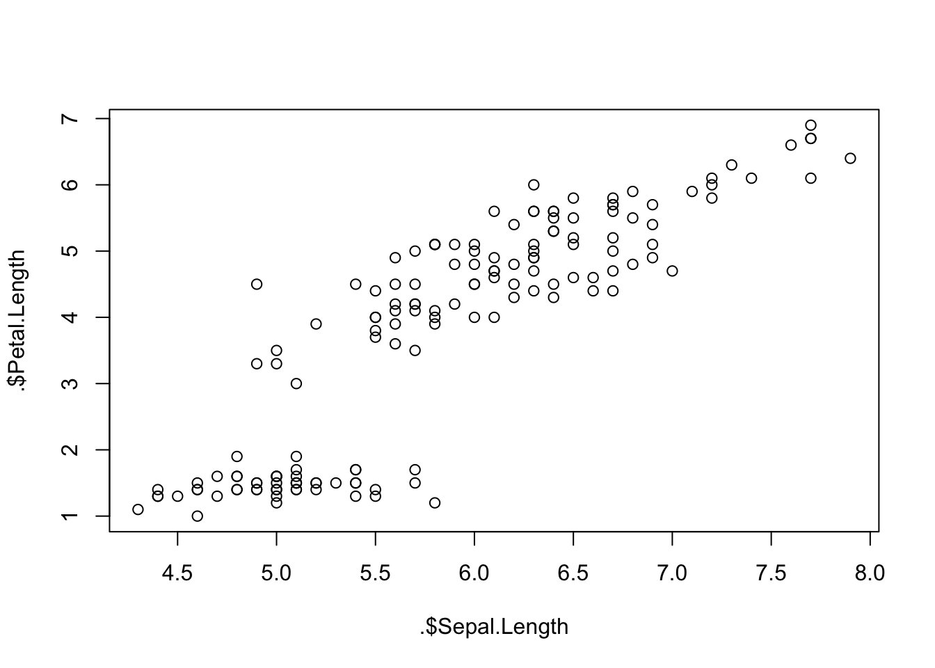
iris %>% {plot(x = .$Sepal.Length, y = .$Petal.Length)}
# which is correctly equivalent to: plot(iris$Sepal.Length, iris$Petal.Length)