Gather Columns into Longer and Narrower Dataset (4/4): Deal with Multiple observations Per Row
So far, we have been working with data frames that have one observation per row, but many important pivoting problems involve multiple observations per row. You can usually recognize this case when the input column names contain both variable names (as they correctly should be) and observation names (which should otherwise be recorded in different rows). In this section, you’ll learn how to pivot this sort of data.
e.g. 1. In the following dataset, each child has two pieces of record, gender and dob (date of birth). child1 and child2 are essentially different observations; instead of occupying different rows as they should be in a tidy dataset, they occupy different columns, rending the dataset not tidy enough.
To tidy up the dataset, child1 and child2 should be cell values in the same column, and gender and dob should be reserved as separate columns. The following script can be conceptualized as pivoting the data at the child level while maintaining the original structure of dob and gender.
family %>%pivot_longer(-family, names_sep ="_", names_to =c(".value", "child"), values_drop_na =TRUE )
names_sep = "_" indicates that the underscore _ is used as the separator to split the original column names into two parts: the part before the underscore, and the part after.
The generic function of names_to = "x" is to turn the input column names as cell values under the x variable. In this case, the second part of the column names, child1 and child2, are turned into cell values under the new column child. The string .value is a special placeholder that, in this case, matches the first part of column names, i.e., dob and gender, and serves two roles: 1) the matched part are reserved as new column names, and 2) .value specifies the values being measured for the new columns in the output (reminiscent to the argument values_to).
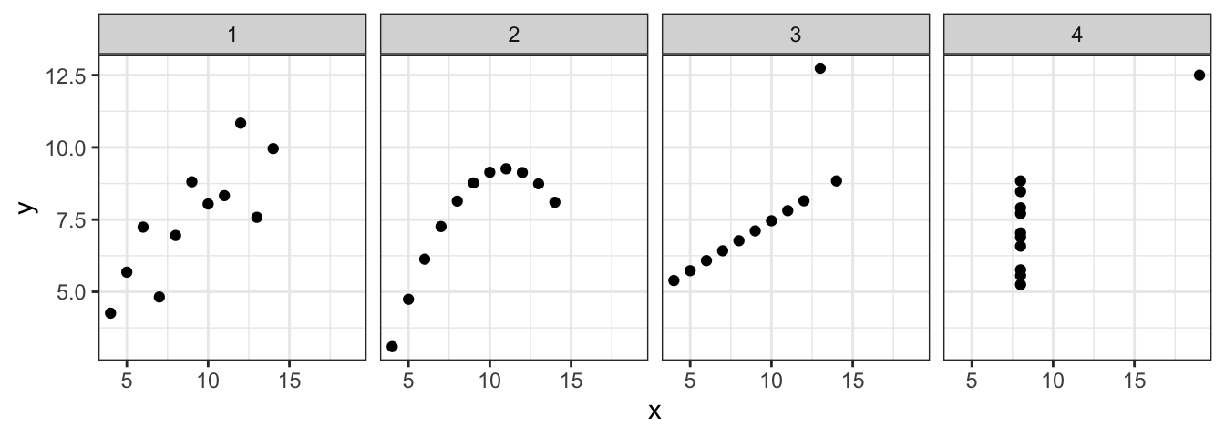
e.g.2. Anscombe’s quartet is a famous example in statistics illustrating the importance of visualizing data distribution rather than relying solely on summary statistics. It consists of four datasets, each containing two variables (x and y). Despite having different data distribution, the four datasets share identical or very similar summary statistics such as mean, standard deviation, correlation, and regression lines. It highlights the importance of visualizing the data distribution, as different datasets with the same summary statistics can have vastly different characteristics.
Below we’ll produce a dataset with columns set, x and y only. For the regular expression(.)(.), each dot is a wildcard representing any character, and the entire expression matches any two single consecutive characters, with each character being an individual capture group.
a <- anscombe %>%pivot_longer(everything(),names_to =c(".value", "set"),names_pattern ="(.)(.)" ) %>%arrange(set)a
To demonstrate the continence brought by the tidy structure, the output can be readily streamlined with ggplot2 to visualize all datasets at the same time.