A Complete Guide on the “brewer” Color Palettes in ggplot2

brewer, distiller, and fermenter

To apply the brewer color palettes, the basic formula is scale_color_* (or scale_fill_*), with * representing three different suffix options: brewer, distiller, and fermenter, depending on the type of the variable that is mapped to the color (or fill) aesthetic.

Categorical variable corresponds to suffix brewer

When a categorical variable is mapped to the color aesthetic, use suffix brewer, i.e., in the form of scale_color_brewer().

# create a scatterplotbase <- iris %>% ggplot(aes(Sepal.Length, Sepal.Width))
base +   geom_jitter(aes(color = Species), size = 3) +  scale_color_brewer(palette = "Accent")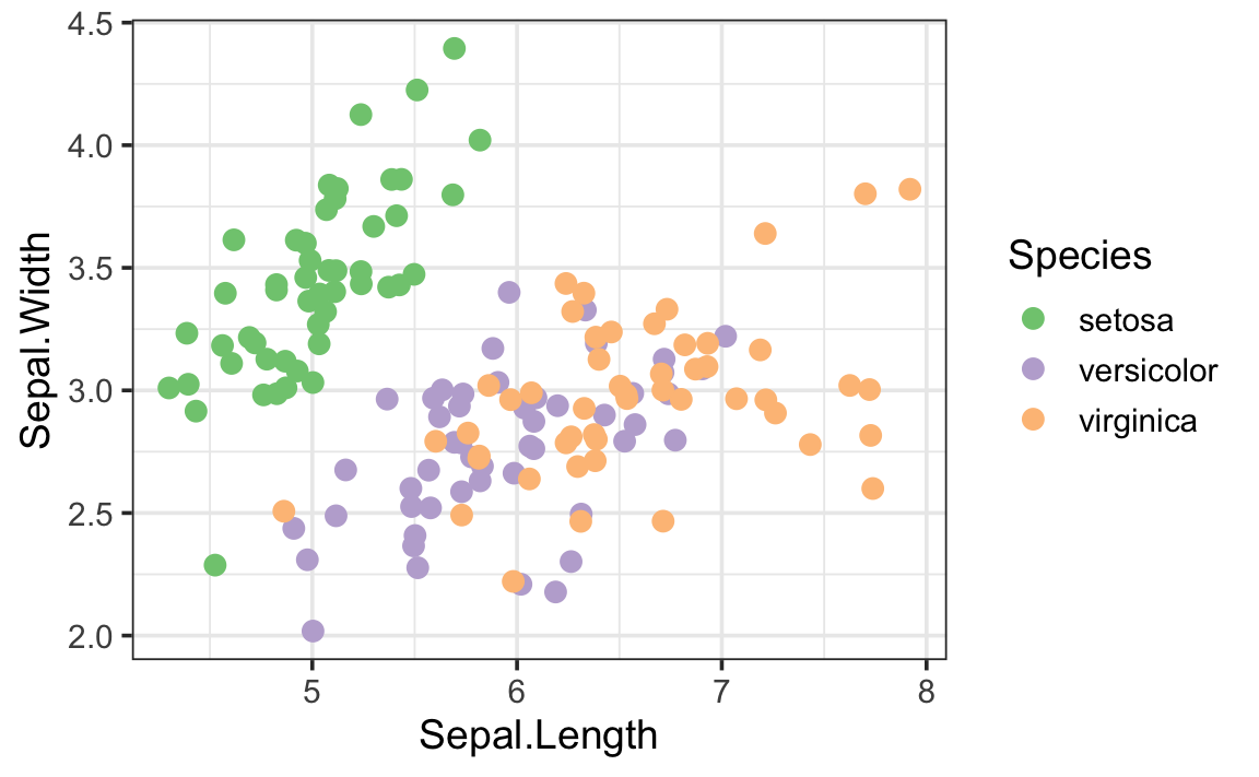

Numeric variable corresponds to suffix distiller or fermenter

When a numeric variable is mapped to color, there are two options:

• use suffix distiller to create a continuous color bar in the legend.

# Petal.Length a numerical variablebase +   geom_jitter(aes(color = Petal.Length), size = 3) +  scale_color_distiller(palette = "Accent")

• use suffix fermenter to create a binned (stepwise) color scale.

base +   geom_jitter(aes(color = Petal.Length), size = 3) +   scale_color_fermenter(palette = "Accent")

When the type of the variable is mismatched with the color scale syntax, it’ll generate an error message typically like: Error: Continuous value supplied to discrete scale.

Display available brewer palettes

scale_color_brewer(), scale_color_distiller(), and scale_color_fermenter() (and the scale_fill_* functions) are all built in the ggplot2 package. However, in order to display the brewer’s available palette names and colors, or to extract colors hex codes from the brewer palettes, you need to additionally load the RColorBrewer package.

The following code displays the brewer’s palette names and colors. It also shows the maximum number of colors available in the palette when a categorical variable is mapped to color (or fill) (see maximum color limit below).

library(RColorBrewer)display.brewer.all()

Extract colors from brewer palettes

After loading the RColorBrewer package, colors can be extracted from a palette and returned as hex codes.

colors.9 <- brewer.pal(n = 9, name = "Set3")colors.9

Output:
[1] "#8DD3C7" "#FFFFB3" "#BEBADA" "#FB8072" "#80B1D3" "#FDB462" "#B3DE69"
[8] "#FCCDE5" "#D9D9D9"

Visualize color hex codes

The scales package offers a solution to visualize the color hex codes.

library(scales)show_col(colors.9)

Maximum color number limit in brewer’s discrete color scale

When a categorical (discrete) variable is mapped to color and scale_color_brewer(), the colors available in the plot is limited by the number of colors in the associated palette. For example, a maximum of 9 colors is available in palette Set 3 (use display.brewer.all() to show available colors; see above). In like manner, when extracting colors using brewer.pal(), no more than 9 colors can be extracted from Set 3.

Note that this maximum color number limit does not apply to scale_color_fermenter() or scale_color_distiller().

This limit in scale_color_brewer() often makes sense, as too many discrete colors (typically used for categorical variables) are difficult to distinguish visually. However, if you do need more colors, you can use the base R function colorRampPalette() to interpolate (generate) as many transitional colors as needed (see below).

Color interpolation

The following code generates 20 colors with smoother color transition from 9 colors of the Set 3 palette.

colors.20 <- colorRampPalette(colors.9)(20) colors.20

Output:
 [1] "#8DD3C7" "#BDE5BE" "#EDF8B6" "#EDECBD" "#D2CFCD" "#C4B3CF" "#DE9BA3"
 [8] "#F78377" "#CD9295" "#99A6BE" "#9AB1BB" "#CEB28B" "#F9B662" "#D9C765"
[15] "#BAD968" "#CAD890" "#E8D1C4" "#F6CEE3" "#E7D3DE" "#D9D9D9"

show_col(colors.20, cex_label = .6)

Demo example: Use color interpolation to overcome maximumm color number limit

stat_density_2d_filled() creates a density heatmap. It divides the continuous density scale into 13 discrete (categorical) intervals, with each interval mapped with a color, and corresponds to color scale scale_fill_brewer(). The Spectral palette, however, can only offer a maximum of 11 colors. This leads to incomplete color mapping in the heatmap and legend.

f <- faithful %>%   ggplot(aes(waiting, eruptions)) +  stat_density_2d_filled() +  coord_cartesian(expand = 0) 
f + scale_fill_brewer(palette = "Spectral")

To generate all the needed 13 colors, we can employ color interpolation to the Spectral palette. Note that the generated colors are supplied to the values argument in the scale_color_manual() function.

myColors <- colorRampPalette(brewer.pal(11, "Spectral"))(13) f + scale_fill_manual(values = myColors)

An alternative solution to color interpolation is to use the popular viridis or scico color palettes, which are never limited to the maximum color number limits.

# viridis palettesp1 <- f + scale_fill_viridis_d(option = "A")
# scico palettes; require calling / loading the packagep2 <- f + scico::scale_fill_scico_d(palette = "batlowK")
library(patchwork)p1 | p2