# Packages and global themelibrary(ggplot2)library(dplyr)theme_set(theme_minimal(base_size = 14))
p <- chickwts %>%   ggplot(aes(x = feed, y = weight))
p + geom_point(size = 3, color = "turquoise4")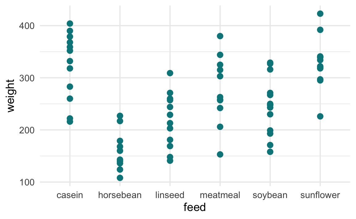
This tutorial explains how to create a scatterplot, covering two critical aspects:
color and fill on the shape aestheticUse geom_point() to create point elements. Each row in the input dataset corresponds to a point in the plot.
# Packages and global themelibrary(ggplot2)library(dplyr)theme_set(theme_minimal(base_size = 14))
p <- chickwts %>% ggplot(aes(x = feed, y = weight))
p + geom_point(size = 3, color = "turquoise4")
position = "jitter" in geom_point() introduces a small amount of random noise to the points’ position, and helps to unveil overlapped data points. The code below allows for additional fine-tune of the amount of randomness in both the horizontal (width) and vertical (height) directions. The seed argument takes any random number, and ensures to reproduce the same randomness each time the code is executed.
p + geom_point( position = position_jitter(width = .1, height = 10, seed = 123), size = 3)
geom_jitter() is a shorthand to create jittered position. However, it does not have the seed argument, which has to be specified via position = position_jitter().
p + geom_jitter(width = .1, height = 10, size = 3)Alternatively, the ggbeeswarm package offers randomization in a more organized and symmetrical manner. It has two major functions, geom_beeswarm() and geom_quasirandom().
# install.packages("ggbeeswarm")library(ggbeeswarm)
# larger 'cex' value makes points more spread apartp + geom_beeswarm(cex = 3, size = 3)
# larger 'width' value makes points more spread apartp + geom_quasirandom(size = 3, width = .2) 
color and fill on shapeIn ggplot2, each shape is represented with a fixed number index. The following script displays the number assignment to each shape.
# create a data frame specifying the coordinate position of each pointd <- rbind(expand.grid(1:5, 5:1),            data.frame(Var1 = 6, Var2 = 1))
# demonstrate points each with a different shapeggplot(d, aes(Var1, Var2)) +  # points of different shapes  geom_point(shape = 0:25, size = 6,              stroke = 2, # thickness of the outline.               color = "steelblue3", fill = "gold") +    # mark the number associated with the shape  geom_text(aes(label = 0:25),             nudge_y = .4,            size = 6, fontface = "bold") +    theme_void() # apply an empty background
shapes 0 ~ 14 are outlines. 15 ~ 20 are solid shapes. All shapes 0 ~ 20 are specified by the color aesthetic .
Shapes 21 ~ 25 each have an outline, specified by color; and an interior, controlled by fill.
To illustrate the dependence of color and fill on the shape aesthetic, compare the following two lines of script. If the feed variable is mapped to fill, instead of color, the points are all black. This is because the shapes in the current plots are sketched in outlines, which corresponds only to the color aesthetic; as such, the shapes do not understand the fill aesthetic.
# colorful pointsp + geom_point(aes(shape = feed, color = feed), size = 3)# black pointsp + geom_point(aes(shape = feed, fill = feed), size = 3)

Shape 21 has both an outline, specified by color aesthetic, and a solid interior, which is controlled by fill aesthetic. In the following plot, the point interior fill is mapped with feed and color-coated, and the outline (not mapped with any variable) takes the default black color. The stroke argument specifies the thickness of borders.
p + geom_point(aes(fill = feed), shape = 21, size = 3, stroke = 1)
Overcrowdedness in scatterplot is a common problem when visualizing large datasets, and makes it difficult to unveil the underlying data pattern. Check out this article to learn powerful techniques to deal with this common issue.

